Hello, this is Mim. I am an artificial intelligence engineer at Ridge-i. I picked the paper titled Exploiting Optical Flow Guidance for Transformer-Based Video Inpainting (FGT++) [1] today to reflect on the progress of deep learning in a challenging vision task: video inpainting.
Introduction to Video Inpainting
Before diving into an explanation of the model, let's get to know what video inpainting is. It’s the same as image inpainting, just the inpainting will happen in the video. Image inpainting typically has the goal of replacing part of a scene, restoring corrupted parts, or filling in the missing parts of an image. A practical example could be removing those annoying watermarks from images or light reflections from medical images. The usage extends to videos too. It’s how the invisible cloak hides Harry Potter – the editor removes the part of Harry’s body from some frames keeping the background as much as possible unchanged. This is for object removal, and the technique can also be applied to video retargeting and other purposes. You can check out the following video if you are interested in some more typical video inpainting examples:
[CVPR2022] Towards An End-to-End Framework for Flow-Guided Video Inpainting [reference: Youtube]
Problem Definition
I have borrowed the problem definition from the first pioneer paper in deep learning-based video inpainting – Deep Video Inpainting (VINet) [2], and other video inpainting papers.
A video inpainting task involves a series of consecutive corrupted frames, denoted as , along with their corresponding masks,
, where N represents the length of the video. Each pixel in a mask Mi is assigned a value of either "0" if the actual pixel value is known (i.e. pixels that should be unchanged ) or "1" if it is missing (i.e. pixels that need to be inpainted). The goal of video inpainting is to use the information from X and M to reconstruct the ground truth sequence
. When preparing the training data, X is typically generated in practice by applying a mask M to a normal video Y, using element-wise multiplication:
In short, the video inpainting problem can be defined as
- Input: Video frames X, and their corresponding masks M
- Output: Inpainted video frames with spatiotemporal consistency Y’
- Spatiotemporal consistency refers to maintaining visual consistency along both pixels and time.
- Ground Truth: Original video frames Y
- Objective: To make Y’ as close as possible to Y
Drawbacks in the Problem Formulation
It is important to note that this problem definition focuses on frame reconstruction rather than object removal because the ground truth data for object removal is scarce as it is labor-intensive and time-consuming to produce. Consequently, datasets specifically for object removal (more specifically in video format) are generally unavailable. According to the authors of RORD [4],
“The common standard for training image inpainting CNNs is synthesizing hole regions on the existing datasets, such as ImageNet and Places2. However, from the viewpoint of the object removal task, such a methodology is suboptimal because actual pixels behind objects, i.e., “ground truth”, cannot be used for training.”
However, that’s how all the current models are being trained.
Common Challenges
In video inpainting, the challenges compared to image inpainting are:
- Temporal coherency: Each pixel does not look weird or too different from previous frames. Otherwise, the video shows flickering or quivering, or jittering which is kind of similar to static noise (vertical lines or small salt-pepper noise) in old TV.
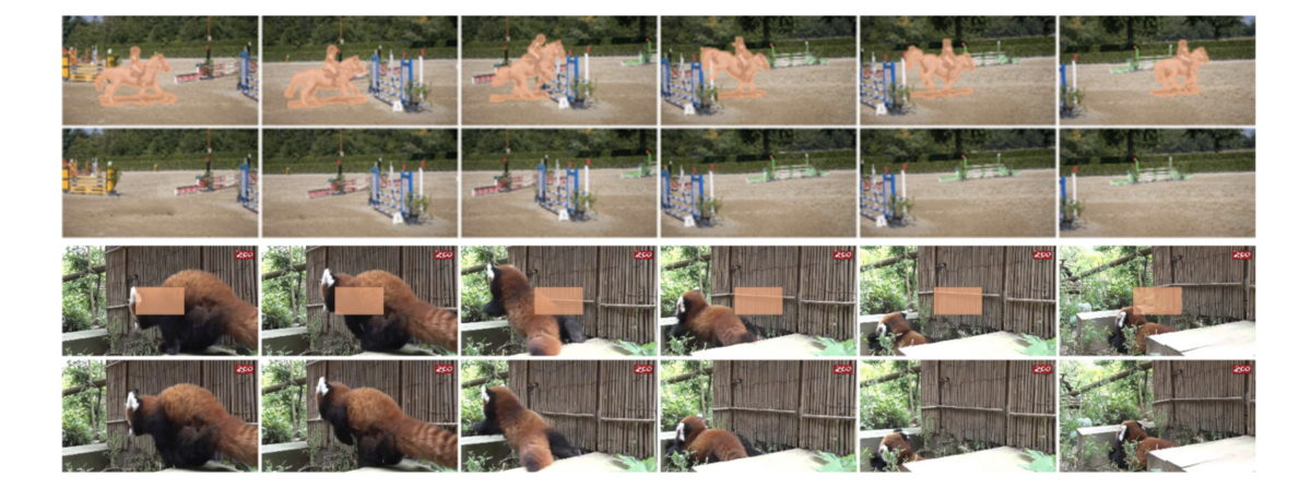
- Dynamic object removal: If the targeted object that we need to remove keeps moving over time from frame to frame, annotating the mask for this object is required for every single frame. So if we have a 2-second video with 30 fps, 60 frames would need to be annotated.
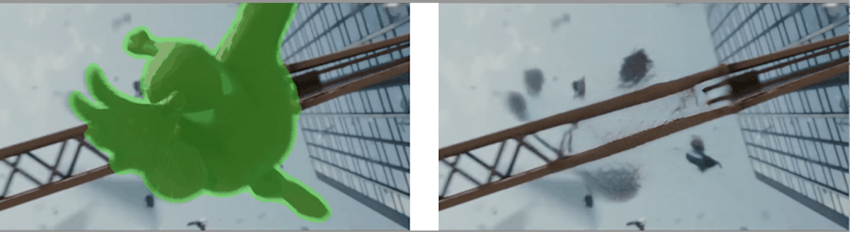
Below is an example of the results of dynamic object removal from Towards An End-to-End Framework for Flow-Guided Video Inpainting (E2FGVI) [5]. The result is not very bad, however, there are still some inherent challenges. It’s noticeable that the last inpainted frame is not temporally consistent i.e. the metal hand coming out of the building has some missing regions after object removal. Additionally, because the Spiderman is moving in each frame, it is necessary to annotate the mask frame by frame (shown in green).
Categories of Existing Models
Video Inpainting papers can be categorized into Flow-Based Models, Learning-Based Models, Combined Models, and, more recently, Diffusion-Based Models. Patch-based models, once innovative, are now largely obsolete due to high computational demands and poor temporal coherence.
Flow-Based Models, though older, are notable for maintaining temporal coherence, while Learning-Based Models, like VINet and DFVI, laid the groundwork for deep learning in Video Inpainting. Given the current landscape, experimenting with both Flow-Based and Learning-Based Models remains worthwhile.
- Flow-Based Models
These models rely on the concept of optical flow, which tracks object movement in sequential video frames. - Learning-Based Models
VINet and DFVI pioneered deep learning in Video Inpainting, with later models building upon their frameworks. Combined Models
This category integrates aspects of both flow-based and learning-based approaches to leverage the strengths of both methods.
FGT++ belongs to this category as it incorporates both flow prediction modules and deep learning architectures and techniques.Diffusion-Based Models
Reflecting recent advancements in generative modeling, these models can belong to any of the above categories and offer promising results in both temporal coherence and detail restoration.
Explanation of Optical Flow
As optical flow and flow prediction serve as important concepts, it’s better to know what they are before jumping into the paper explanation. If you already have the idea, feel free to skip this part. Let’s think a bird is flying and you are capturing a video of its flight. For simplicity, imagine the camera is mounted on a tripod and it’s not moving at all. How will this flying motion appear in the video? The bird’s location in each frame will keep changing! If we would like to calculate the birds’ flying speed, it will be:
/
where,
is the starting time
is the end time
is the position at
is the position at
However, we do not say it is the actual motion of the bird, rather we call it apparent motion because the distance is measured in pixel space, not in actual space. This motion is optical flow.
And what is flow prediction? It is the prediction of the optical flow of different pixels in such cases:
- Some pixels are corrupted or missing
- Consecutive frames are corrupted or missing
Check out this video if you want to learn more about optical flow and the maths behind it:
Optical Flow Constraint Equation | Optical Flow [reference: Youtube]
Paper Explanation
FGT++
Github: https://github.com/hitachinsk/FGT
License: MIT license
Is pre-trained weight public: YES
The latest model in the FGT series is FGT++, which claims to outperform the Transformer model from E2FGVI. A Summary of E2FGVI will be given in the next section. To eliminate any confusion, I will explain the FGT++ paper, which is the journal extension of FGT and features a slightly different architecture. FGT++ is a more advanced version compared to FGT [6].
Please check the simplified version of the FGT++ model architecture for a better understanding.
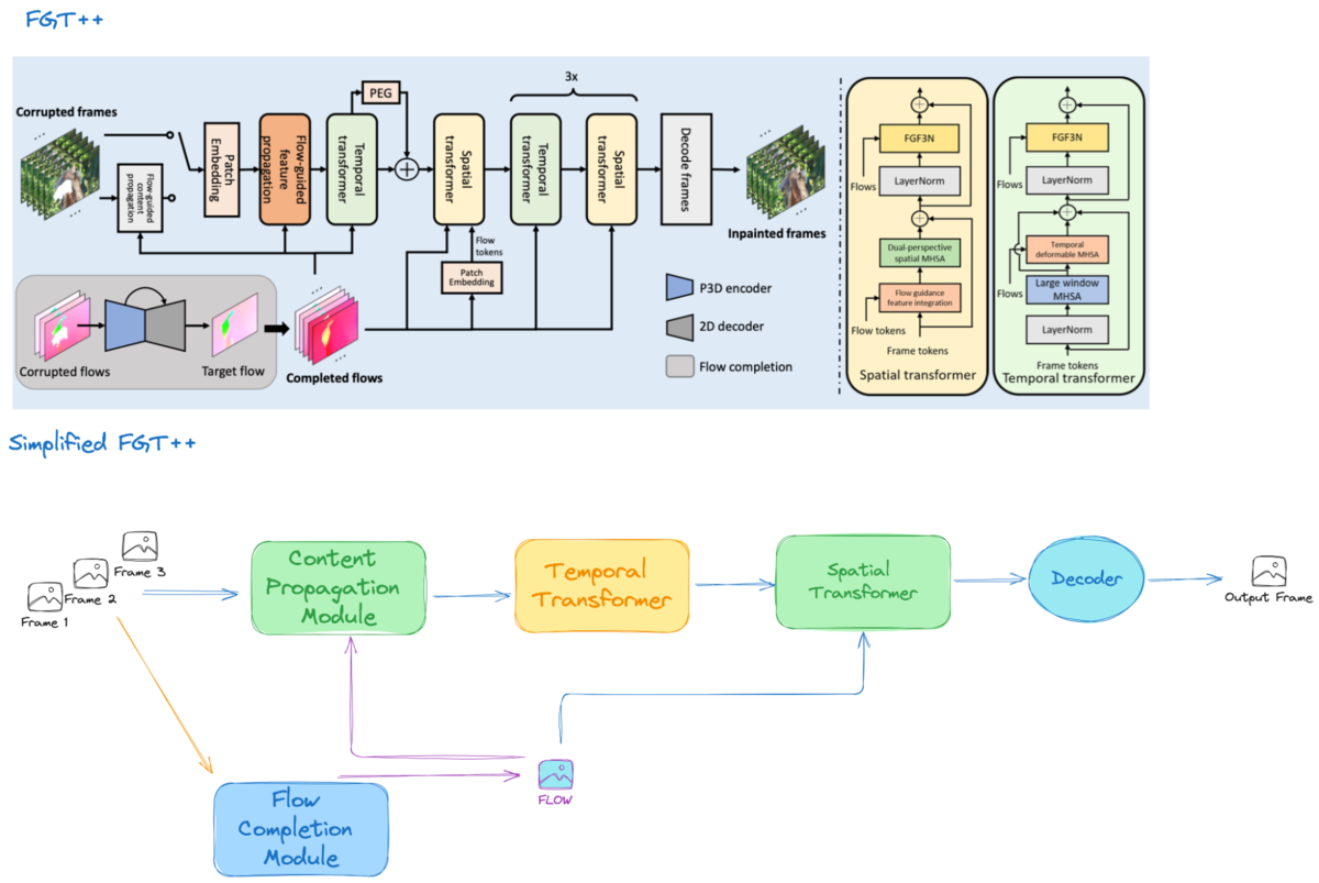
At a glance, the architecture of FGT++ begins with a flow completion module. On top of FGT, FGT++ uses a more nuanced flow completion network to produce high-quality flow maps of frames. These high-quality flows are then fed into the content propagation module, along with local frames (reference frames, lagging frames, and leading frames) and some far-reaching global frames.
Next, the tokens enriched with flow from the content propagation module pass through a Temporal Transformer and a Spatial Transformer. In the Temporal Transformer, techniques like large window attention are employed for a large receptive field along the temporal axis. However, since this large window obstructs the learning of small neighboring correlated relations, deformable multi-head self-attention (MHSA) [7] is used on top of the large window MHSA. Afterward, these tokens go through the Spatial Transformer, where flows are included to guide features to spread spatially coherently. Finally, a decoder is used to produce the final inpainted output.
During the training of FGT++, in addition to the standard reconstruction loss, warp loss, and GAN loss, a frequency domain loss (i.e. FFT loss) is included. FFT loss has been added to supervise the amplitude of the Fourier transform between the reconstructed frames and the ground truth.
The flow completion network also introduces edge loss. Optical flow estimation models typically struggle with boundary regions and edge loss is used to address this. Edge loss, as the name implies, is a specialized penalty that preserves sharp boundaries by comparing the inpainted edges against the ground truth. In FGT++, this loss term ensures not only pixel-level accuracy but also edge consistency, helping maintain fine details and prevent the blurring or smearing of object outlines across video frames. Edge Loss is calculated as:
where,
represents the Binary Cross Entropy Loss
represents the Canny Edge Detector
is the ground truth flow at time t
is the predicted flow at time t’
Since edge loss has been applied in previous papers, the novel contribution of this paper is local aggregation in the flow completion module. Local aggregation is used to improve flow estimation by leveraging the correlation between motion fields of consecutive frames, which is influenced by the physical principle of inertia. This approach can be seen as an example of Physics-Informed Neural Networks, where physics equations aid in the convergence of neural network models.
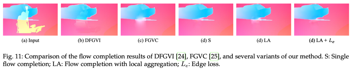
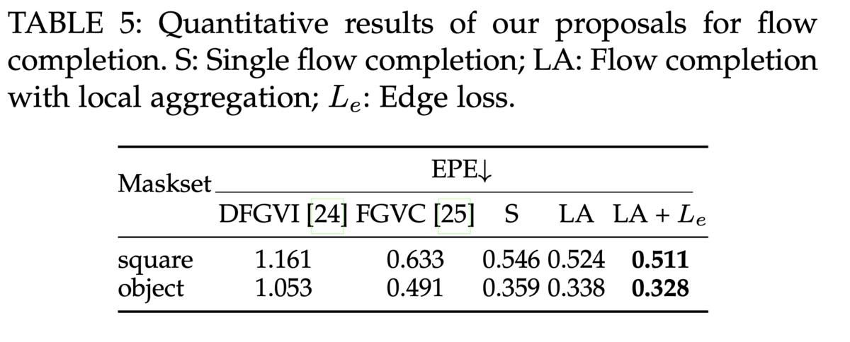
The figure below illustrates the qualitative improvements that FGT++ achieves by incorporating both edge loss and local aggregation. The first table presents the EPE loss (which is commonly used in evaluating the task of flow prediction) for flow completion on the DAVIS [8] dataset (square and object). The images below show the optical flow outputs generated by the flow prediction network. Generally, higher-quality flow completion leads to better video inpainting results. For example, the optical flow predictions from DFVI (or DFGVI) and FGVC [9] exhibit blurring and smearing around edges, whereas the variant of FGT++ produces smoother, well-defined edges in its flow predictions.
FGT++ also solves the query degradation problem, where masked regions suffer from degraded features in MHSA blocks. This is addressed by incorporating optical flow, which helps propagate information from previous frames to improve feature quality in these areas. Additionally, FGT++ enhances the process by integrating flow guidance during tokenization, improving the handling of masked regions.
2021 SOTA Model E2FGVI
Github : https://github.com/MCG-NKU/E2FGVI
License: CC BY 4.0
Is pre-trained weight public: YES
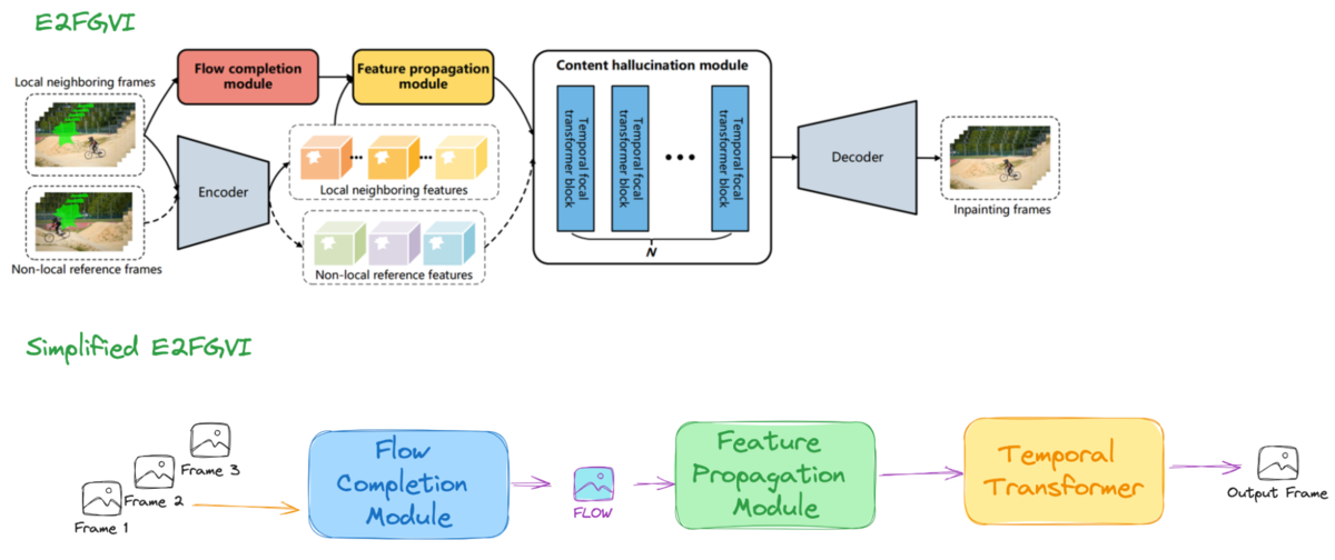
Conventional video inpainting performs flow+propagation+inpaint independently in the pixel space, which is a bottleneck in terms of accuracy and speed. Instead, E2FGVI performs inpainting end-to-end in the feature space. The overall architecture is shown below, where the flow is calculated using a pre-trained lightweight Optical Flow Estimation using a Spatial Pyramid Network (SPyNet) [10], being applied to the encoded features. The warped results are bidirectionally combined, and finally, the features are inpainted with a focal Transformer and then decoded.
Using the YouTube-VOS [11] and DAVIS datasets, the author compared their method with existing methods and demonstrated its superiority through various evaluation metrics and user studies.
FGT++ vs. E2FGVI
Comparison Summary
| Model | FGT++ | E2FGVI |
|---|---|---|
| Main Structure | Flow-Guided Transformer | End-to-End Flow-Guided Video Inpainting |
| Temporal Coherence | Better than E2FGVI | Good |
| Dynamic Object Removal | Better than E2FGVI | Good |
| Training Data | Synthesized masks | Synthesized masks |
| Pre-trained Weights | Available | Available |
| License | MIT | CC BY 4.0 |
| Application Examples | Watermark removal, object removal, video retargeting, video extrapolation | Object removal, video completion |
| Optical Flow Integration | Yes | Yes |
| Performance on Benchmark Datasets | Superior | Good |
Architecture Improvement
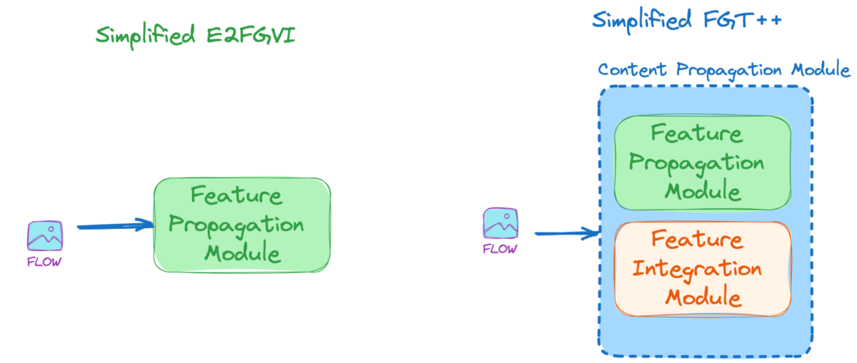
To find out the architectural improvement of FGT++ from E2FGVI, let’s analyze the simplified model version of FGT++. It is evident that the optical flow guidance is utilized more extensively in FGT++ than in E2FGVI. In FGT++, it is employed in both the Spatial and Temporal Transformers, whereas in E2FGVI, it is limited to the Spatial Transformer. Theoretically, the FGT++ model will be more spatially and temporally coherent.
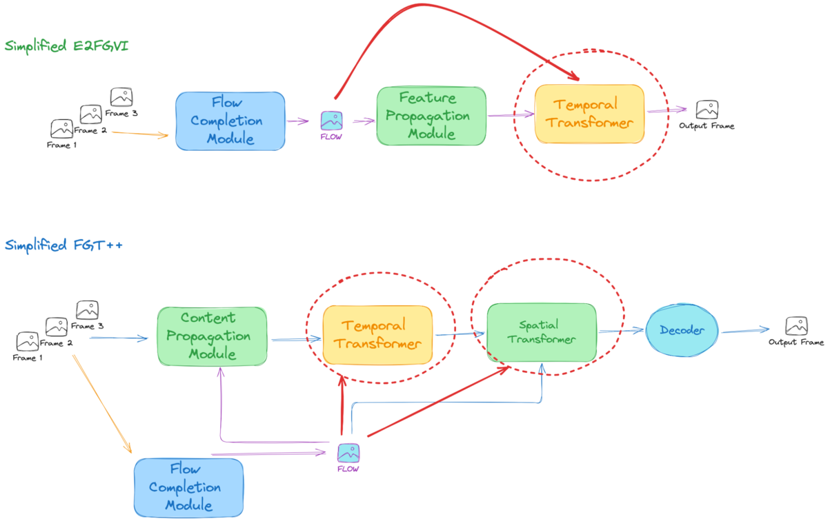
The flow propagation module has also been improved with additional elements. In E2FGVI, we have a feature propagation module to propagate features with optical flow guidance. However, in FGT++, besides the feature propagation module, the so-called feature integration module has been added, both of which form a content propagation module.
Improved Optical Flow Estimation Model
As for the optical flow estimation model, E2FGVI uses SPyNet which is lightweight and efficient, and FGT++ uses RAFT [12] which is the latest top-performing lightweight model.
Qualitative Proof of Improvement
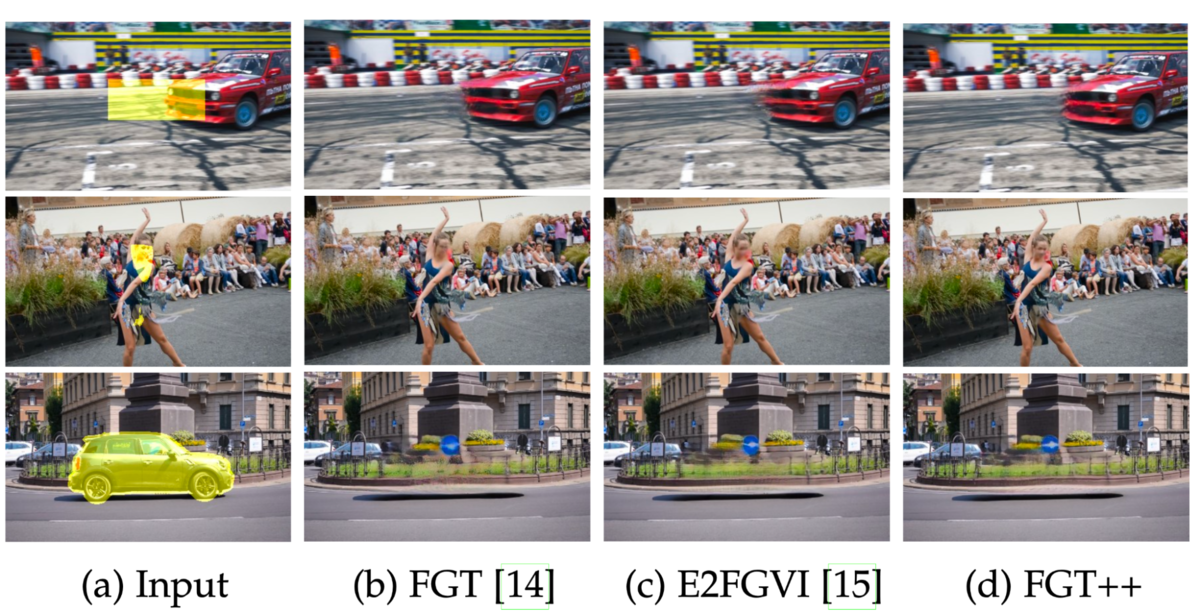
From the inference examples of FGT++ and E2FGVI, it seems FGT++ is better at reconstructing human faces (which is one of the most frequent domains of practical applications, including pedestrian and industrial labor monitoring).
Drawbacks
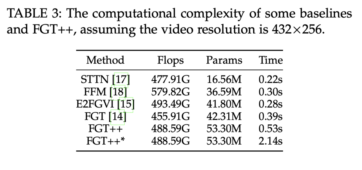
The following table shows how much time each model takes to infer one frame. Even though FGT++ has better performance than E2FGVI, it has a longer inference time. FGT++* is the slowest due to poisson blending at the post-processing stage. It is therefore kind of a trade-off between the speed and realistic video generation quality.
Conclusion
In the domain of video inpainting, rapid and significant advancements have emerged following the adoption of deep learning techniques. Among the state-of-the-art models, both FGT++ and E2FGVI are commendable when considering factors such as licensing restrictions, availability of training code, and publicly accessible pretrained weights. However, when evaluating flow completion results — which are crucial for achieving optimal performance in video-related tasks — FGT++ demonstrates superior effectiveness.
References
- Exploiting Optical Flow Guidance for Transformer-Based Video Inpainting
- Deep Video Inpainting
- Deep Flow-Guided Video Inpainting
- RORD: A Real-world Object Removal Dataset
- Towards An End-to-End Framework for Flow-Guided Video Inpainting
- Flow-Guided Transformer for Video Inpainting
- Attention is All You Need
- DAVIS
- Flow-edge Guided Video Completion
- Optical Flow Estimation using a Spatial Pyramid Network
- YouTube-VOS
- RAFT: Recurrent All-Pairs Field Transforms for Optical Flow