Did you know that denoising is the only technology from Disney Research that gets special thanks in the credits of Frozen II ?
Denoising technology has been used in every single Pixar movies ever since Toy Story 4 (2019). In this article, I'd like to share how Pixar is currently using deep-learning to produce high-quality animation that would not be possible without it.
The rendering bottleneck
What is rendering
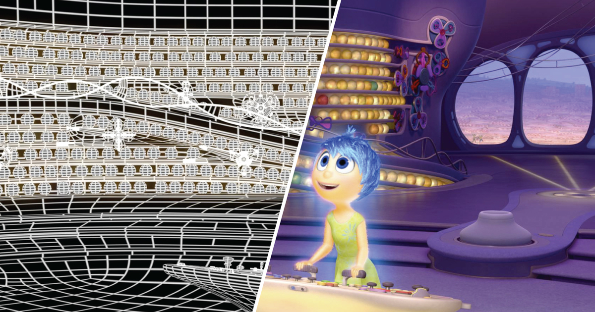
Rendering is the process of turning a 3D scene into a 2D image.
After characters, objects, light sources and cameras positions are defined in the 3D scene, the value of each pixel of the final image is computed by simulating how the light from each source (color, intensity, angle etc) will bounce on each element (considering material, texture etc) of the scene.
Light simulation
Given a light source, a scene and a camera, there are two main methods to compute the illumination received by the camera :
Forward tracing : In real life, light sources emit photons that bounce on objects until they reach the camera. Forward tracing is similar to real life behavior as rays are launched from light sources and bounce on the scene's elements until they they reach the camera and used to compute illumination at each output pixel. The main drawback is that simulation is slow as most rays emitted by the lights will never even reach the camera.
Back tracing : Instead of tracing rays from the light source to the camera, rays are traced backward from the camera to the objects. If the ray hits an object, additional rays are thrown from the impact point until we reach the light source. It is often preferred to photon mapping as it is faster to render (only rays that will eventually reach the camera are computed) at a cost of quality when encountering highly reflective or refractive surfaces (like mirrors and glass) that cause "caustics".

Some surface like glass can concentrate light and prevent some regions from ever being reached source
| Forward tracing | Backward tracing | |
|---|---|---|
| Advantage | Photo-realism | Faster to render (only rays that will eventually reach the camera are computed) |
| Drawback | Very slow (rays are randomly emitted by the light sources, even ones that will never reach the camera) | Due to some surfaces (like glass), some regions will never be reached |
To take advantage of both methods' strengths, hybrid methods (such as bidirectional path tracing) are used. They are faster than forward tracing but don't suffer as much as back-tracing from surfaces like glass.
The amount of rays used for simulation can be set by the user through the number of "iterations". More iterations = better quality images.

The issue
The rendering process is extremely time consuming. It takes about 24 hours to render a single frame which means that a 100 min movie would take about 400 years ! According to Pixar, even with 2000 machines and 24,000 cores, it still took 2 years for Monster University (2013) to fully render.
It usually takes 4 to 7 years to complete a Pixar movie but out of those years, up to half are spent solely for rendering !
How can deep-learning help reduce this bottleneck ?
Denoising with deep-learning
An unfinished rendering simulation looks like a noisy image with black pixels noise called "Monte Carlo" noise. As such, it is possible to "denoise" an unfinished simulation into the final 2D image.

The field of image denoising is currently dominated by deep learning methods where the model learn from pairs of images (clean, noisy). Using their past movies, Disney has built datasets of (clean images, noisy images) and managed to train models that can generalize well to other movies.

Architecture used
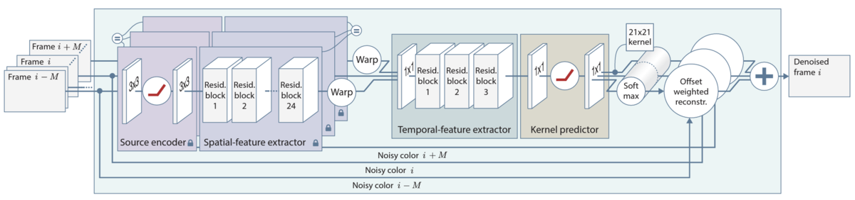
The model currently used by Pixar has been roughly the same since 2018 with no major changes. Their architecture is described in their paper "Denoising with Kernel Prediction and asymmetric Loss Functions" at SIGGRAPH2018.
Modules description
Source encoder : Extracts a low-level representation of the image. Data obtained from different softwares (RenderMan at Pixar / Hyperion at Disney) might have small differences in how the image is rendered which is why multiple encoders (one per renderer source) are fine-tuned from a common denoising back-end to achieve a common representation. The retrained part only consists in two 3x3 convolutional layers which make it very fast to adapt the denoising model to new sources.
Spatial-feature extractor : Extracts spatial features from one input frame. To avoid optimization instabilities, residual blocks are used and were shown to improve performance significantly. Features from different frames are warped and concatenated to make sure that the content from each frames are aligned using motion vectors (usually given by the renderer).
- For example if character at position (0,0) in frame 0 moves to (1,1) at frame 1 and (2,2) at frame 2, the features from frames 0 and 2 are warped to align on the middle frame at (1,1).
Temporal-feature extractor : When denoising successive frames independently, a "flickering" effect can be observed. This is because each of the denoised frames is “wrong” in a slightly different way. Using multiple frames, consistency can be achieved. At each pixel, the multiple kernels computed from each frames are jointly normalized using a softmax.
Multi-scale denoising : Denoising models are good at removing high-frequency noise but usually leave some low-frequency noise. To tackle this issue, the input image can be down-sized (3 times with 2x2 down-sampling in this case) and the denoised results from different scales can be combined progressively (from coarse to fine). Weights at each pixel used to blend two images are predicted using a CNN.
Asymmetrical loss
As a baseline, the Symmetric mean absolute percentage error (SMAPE) loss is used. This choice is motivated by the possibility for the user to specify the level of residual noise ε we want to retain for artistic reasons (trying to completely eliminate residual noise often leads to blurry images and low level of detail).

An improved "asymmetrical" version of this loss was proposed to further allow the model to retain some of the initial noise from the input when the minimum loss can not be reached.

If the differences (d − r) and (r − c) have the same sign (= the filtered result and the input are not on the same “side” relative to the reference), we penalize the result by multiplying the original loss ℓ by the slope parameter λ. Given two solutions that are equally close to the ground-truth image, the model will favor the solution that deviates the less from the input.
Performance
Compared to existing denoiser (N-DP and NFOR), the model was shown to achieve very good performance.

However, as explained in the paper, lower residual error doesn't mean better looking image. As such, more recent models that outperforms this model and have lower residual errors might not actually produce better "artistic" result.
Runtime cost
The denoising cost is 10.2s per 1920 x 804 frame with a 7-frame temporal denoiser, 21x21 kernel prediction on a Nvidia Titan X GPU.
The breakdown is as follow :
- Spatial-feature extractor : 3s
- Temporal combiner : 2s
- Kernel prediction : 5.2s
Using this method, we can render a frame in 10.2s instead of 24h !
Try it ourselves
In this part, we will share how to reproduce the process ourselves : Make something in 3D → Unfinished simulation = Noisy image → Denoise the image (Intel® Open Image Denoise)
First of all, we use Blender to make a 3D model of something

Rendering can be done directly in Blender. Since our scene is very simple, even with few steps, decent results can be achieve. (As reference, 100 iterations take about 3 minutes on CPU).

Denoising with Intel® Open Image Denoise can be done directly inside Blender or by downloading the code from the official website (https://www.openimagedenoise.org/) or their GitHub (https://github.com/OpenImageDenoise/oidn).
Running the result of one iteration, we successfully denoise the image without any visible artifacts.

The results (obtained in few seconds) is visually better than the rendering running for about 1h (2000 iterations) which still has some noise on the metallic texture of the mug.

Conclusion
Denoising technology has helped Pixar cut down the time needed to render images from multiple hours per frame to few seconds. Not only has it helped cut down costs and resources needed, it also allowed team to work in better conditions as animators and artists can now simulate what their work would look like in the final product and adjust accordingly.
Is it faster to make movies now ?
No. Instead, Pixar has taken this opportunity to add more and more details and constantly comes up with new challenges to tackle.

In addition to denoising, other deep-learning based method have been used by Pixar to further improve the quality of their movies (GANs with super-resolution etc)
References
Papers :
- https://graphics.pixar.com/library/MLDenoising2018/paper.pdf
- [PDF] RenderMan: An Advanced Path-Tracing Architecture for Movie Rendering | Semantic Scholar
- [1912.13171] Deep Learning on Image Denoising: An overview
- Denoising with Kernel Prediction and Asymmetric Loss Functions – Disney Research
- Machine Learning Denoising In Feature Film Production
OpenImageDenoise by Intel:
Blog articles and others :
- Deep Rendering | Disney Research Studios
- How Disney's 'Frozen 2' Was Animated
- Pixar's RenderMan | Stories | Pixar's USD Pipeline
- Rendering | The Science Behind Pixar
- Ask a Pixar Scientist | The Science Behind Pixar
- How Pixar's Animation Has Evolved Over 24 Years, From ‘Toy Story’ To ‘Toy Story 4’ | Movies Insider - YouTube
- How Pixar Uses AI and GANs To Create High-Resolution Content « Machine Learning Times
- Frozen II Credits | Walt Disney Animation Studios Wikia | Fandom